Simulation and the waveform
yanc stops at the Verilog (see The command line). The
output folder then holds everything a simulator needs: the processor
<name>.v, its memories, and the testbench <name>_tb.v, which feeds each
input port from input_N.txt beside the source and writes what the program
outputs to output_N.txt. This page runs it with Icarus Verilog or
Verilator and opens the waveform in GTKWave.
Simulating with Icarus
From the output folder, with SAPHO the SAPHO/ folder that comes with
YANC (on Windows, in the MSYS2 UCRT64 terminal, written /c/path/to/SAPHO
for C:\path\to\SAPHO; see Installing YANC):
export SAPHO=/path/to/yanc/SAPHO
cd my_program
iverilog -s my_program_tb -o sim.vvp -y "$SAPHO" my_program_tb.v my_program.v
vvp sim.vvp
cat output_0.txt
-y "$SAPHO" makes the simulator look in SAPHO/ for each module it is
missing, in the file of the same name: processor in processor.v, and
from there core.v, ula.v, addr_dec.v, instr_dec.v, and myFIFO.v
or myDCFIFO.v when a project uses them. Listing the files instead works
too.
The testbench simulates as many clocks as yanc -c said (10000 by
default) at the clock of yanc -f (100 MHz by default), and writes the
waveform to my_program_tb.vcd.
Run the simulation from the output folder. The generated Verilog names
every file relative to it: the memories (my_program_inst.mif,
my_program_data.mif), the PC table, the outputs (output_N.txt,
toma_k.txt) and the waveform by their bare names, and the inputs
(input_N.txt, cade_k.txt) by the way from the output folder to the
source, ../input_0.txt when the output folder is the default one beside
the source. No absolute path is written, so the folder can be moved or
copied to another machine along with the source, and a folder name with
accents or spaces costs nothing: the YANC tools work in UTF-8 on Windows,
Linux and macOS alike. To synthesize, give the synthesis tool the .mif
files in its project folder, or their full path in the DFILE/IFILE
parameters.
What you see in GTKWave
Because the toolchain emits a side-table mapping each PC value to its originating C± source line, GTKWave shows the executing C± line, the assembly opcode, and every declared variable evolving in lockstep with the simulated clock — not just raw bus toggles:
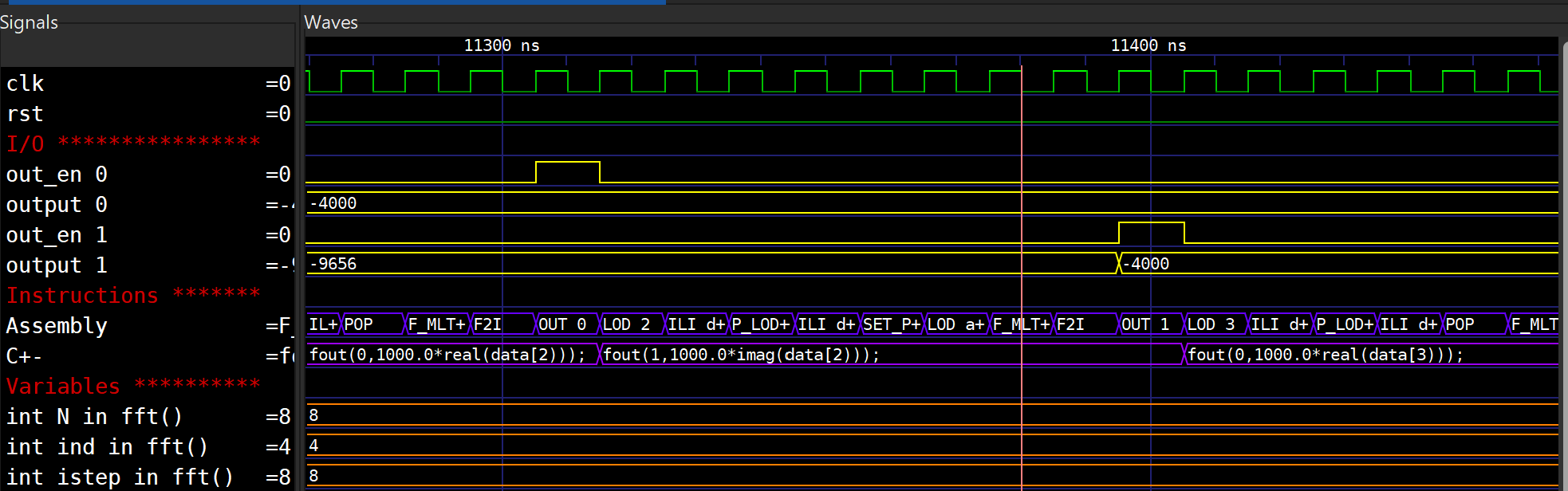
The example above is proc_fft mid-run: the C± track shows the
fout(0, 1000.0*real(data[2])); statement, the assembly track shows
the matching LOD / F_MLT+ / F2I / OUT 0 sequence, and the
declared variables (N, ind, istep, j, k, m, mmax,
sind, comp temp) carry their live values.
Simulating with Verilator
Verilator 5 compiles the same generated <proc>_tb.v directly — --timing understands the testbench’s clock and # delays, so no separate C++ driver is needed:
# from the output folder, my_program/
cd my_program
verilator --binary --timing --trace +define+YANC_TRACE --timescale 1ns/1ps \
          --top-module my_program_tb -Wno-lint -Wno-MULTIDRIVEN -Wno-BLKANDNBLK \
          -Wno-COMBDLY -Wno-STMTDLY -Wno-INFINITELOOP -Wno-UNOPTFLAT --Mdir vl \
          -y "$SAPHO" my_program_tb.v my_program.v
./vl/Vmy_program_tb     # runs the sim, writes my_program_tb.vcd here
gtkwave my_program_tb.vcd
On Windows, MSYS2’s gcc 16 needs -CFLAGS -D_GLIBCXX_ASSERTIONS added to
the verilator line, or the link fails (see
Installing YANC); the scripts below add it
themselves.
--timescale 1ns/1ps gives the SAPHO modules the testbench’s time unit:
the files -y finds are read on their own, so they do not inherit the
testbench’s `timescale as files listed after it do, and Verilator
stops at the difference.
Verilator builds with GNU make, which refuses a build folder whose path has a
space. If the output folder’s has one, point --Mdir somewhere without
spaces and still run the binary from the output folder.
The one thing to remember: +define+YANC_TRACE is what makes your variables, arrays, the PC→C± line table and the assembly opcode appear in the waveform. Icarus gets them for free (it predefines __ICARUS__); Verilator only compiles that visibility harness when you pass the define. For big multi-millisecond project dumps, use --trace-fst instead of --trace (compact FST; the file is still named <tb>.vcd and GTKWave detects the format). The trace deliberately carries only the <proc>-level user signals — the CPU internals below each processor are fenced out with /* verilator tracing_off */. In particular the stack-monitoring flags and the ULA rounding-error taps (fl_max, fl_full, pointeri, delta_int, delta_float) are intentionally not in the Verilator VCD: keeping them would force Verilator to evaluate the expensive real-valued ULA monitoring logic every cycle, which defeats the whole point of using Verilator (speed). Those debug signals remain available under the Icarus flow (Scripts\single_proc.bat / multi_proc.bat), where raw speed is not the goal.
Formatting the waveform — gen_gtkw (optional)
After simulating with either Icarus or Verilator you have a raw <tb>.vcd /
.fst: every signal, in scope order, unformatted. If you want the curated view
instead — the input/output ports, the Assembly and C± instruction
tracks (disassembled through their translate files), and the internal
variables and arrays grouped per processor — run gen_gtkw (it is in the
release’s bin/), then open the waveform with it applied via -a. From the
Quick start’s output folder:
gen_gtkw my_program_tb.vcd my_program_tb.gtkw ..
gtkwave my_program_tb.vcd -a my_program_tb.gtkw
gen_gtkw reads only the VCD header (the signal list), classifies each
harness signal by name, and writes a formatted .gtkw save file: the right data
format / colour / alias per signal, the trad_opcode.txt / src_lines.txt
translators on the Assembly / C± tracks, comp2gtkw.exe on complex signals, and
one section per processor — any scope that owns both valr2 and linetabs — so
the same tool handles single- and multi-processor dumps. Its third argument
is the folder that holds each processor’s output folder, where its translate
files are (.. from inside my_program/ in the Quick start, the folder that
holds my_program/). When the output folder is not named after the
processor (yanc -o build, an .asm in a folder of another name), give the
output folder itself: . from inside it.
Because only the header is needed, the big project FST dumps don’t have to be
written in full first: run the sim once with the +HEADER_ONLY plusarg and
the testbench dumps the header, advances one tick, flushes and $finishes — a
tiny header VCD in milliseconds (Verilator’s header FST is converted with
fst2vcd -f). The runner scripts wire this whole sequence up
correctly (header pass → gen_gtkw → gtkwave -a), so they are the reference
for using it in practice. They also open GTKWave with --dark, and with
--zoom-fit (the whole trace in the window) and --left-justify when that
GTKWave lists them, as the nipscernlab build does (see
Installing YANC).
Pre-wired scripts
Three scripts in the repository’s Scripts/ folder run the whole way, from a test program to GTKWave, with sensible defaults. Each has a
Windows (.bat) and a Linux (.sh) version, and picks the simulator from a
--sim iverilog|verilator flag (default Icarus):
Scripts\single_proc      .bat / .sh   one C± processor    (edit PROC / FNAM at the top)
Scripts\multi_proc       .bat / .sh   C± multi-proc project
Scripts\single_proc_cpp  .bat / .sh   one C++ processor   (front end: cppcomp)

  ... default (no flag)        -> Icarus Verilog (iverilog + vvp)
  ... --sim verilator          -> Verilator (--binary --timing, +define+YANC_TRACE)
  ... --no-view                -> (single_proc_cpp) run the pipeline, skip GTKWave
In the UCRT64 terminal on Windows, as on Linux, run
Scripts/single_proc.sh (or Scripts/single_proc.sh --sim verilator); on
Linux make them executable once (chmod +x Scripts/*.sh). The .bat
versions do the same from cmd.
The C++ runner (single_proc_cpp) feeds a .cpp program — the bundled
Compilers/CPPComp/Tests/proc_cpp demo — through cppcomp instead of
cmmcomp, then the same assemble / simulate / view back end. cppcomp now emits
the same files cmmcomp does (the .asm, prog_log.txt, the pc_<proc>_mem.txt
PC→source line table and src_lines.txt), so the waveform looks just like the C±
flow — with one rule: GTKWave only shows C++ variables that live at a fixed
data-memory address, because the dump snoops a constant write address
(if (mem_addr_wr == X)). That covers globals, the locals/params of
non-recursive functions, and static locals — int shown as a raw word, float
decoded, arrays element-by-element, exactly as in C±. Stack-frame locals of
recursive functions (no fixed address), pointers (an address, not a value) and
structs (a multi-word aggregate) are deliberately not traced. This mirrors
C±, which — for optimization reasons — only ever allocates fixed-address
variables anyway, so both flows show the same kind of thing.